Calculating statistics from boxscores

While boxscores record the important on-court actions in a convenient way, to analyse both player and team performance, it is useful to calculate more advanced statistics. The aim of this Chapter is to calculate some advanced stats from the data in a boxscore CSV file, and carry out some analysis of these stats.

As usual, we start by importing the modules and libraries we will need.

from pathlib import Path
import datetime as dt
import pandas as pd
import matplotlib.pyplot as plt

We are now going to create a dataframe from the boxscores of the Sheffield Hatters vs Caledonia Gladiators game that took place on 27 October 2024. The CSV file containing this boxscore was created using similar code to that shown in the Chapter on scraping boxscore data.

The CSV file is also available to directly download.

Note that you calculate most of these statistics in spreadsheet software, if you would prefer.

path_to_file = Path('data/Hatters-Vs-Gladiators-20241102.csv')
if path_to_file.exists() and path_to_file.is_file():
    boxscores_df = pd.read_csv(path_to_file, index_col=0)
else:
    print("Unable to open the file:", path_to_file)

Let’s have a quick peek inside the file to make sure it contains what we expect.

boxscores_df

	Name	Team	Mins	PTS	FGM	FGA	FG%	2PM	2PA	2P%	...	DREB	REB	AST	TO	STL	BLK	BLKR	PF	FOULON	PLUSMINUS
0	L. Zolper	Hatters	29:00	12	2	8	25	1	5	20	...	3	3	1	3	2	0	0	1	4	5
1	G. Gayle	Hatters	23:55	16	4	7	57	3	6	50	...	2	2	2	1	1	0	0	4	7	12
2	N. Krisper	Hatters	33:37	15	6	10	60	5	7	71	...	1	5	5	5	2	0	0	3	3	10
3	M. Washington	Hatters	31:36	12	6	9	66	6	9	66	...	4	6	4	3	5	1	0	2	2	13
4	E. Gandini	Hatters	20:30	2	1	4	25	1	2	50	...	6	6	1	1	0	0	0	1	1	10
5	M. Emanuel-Carr	Hatters	11:01	7	2	4	50	2	4	50	...	1	1	3	2	1	0	0	1	2	7
6	C. Drennan	Hatters	18:13	9	3	3	100	1	1	100	...	0	0	1	1	0	0	0	3	4	-2
7	E. Nibbelink	Hatters	5:17	0	0	0	0	0	0	0	...	1	1	0	1	0	0	0	0	0	1
8	S. Harrison	Hatters	17:21	7	3	8	37	3	6	50	...	4	4	1	1	0	0	1	2	2	-2
9	L. Wright-Ponder	Hatters	9:30	6	3	6	50	3	6	50	...	1	4	0	3	0	0	0	5	1	-4
10	M. Domenger	Gladiators	22:47	8	2	6	33	2	4	50	...	3	5	3	4	0	0	0	4	3	-3
11	H. Robb	Gladiators	23:43	2	1	4	25	1	2	50	...	2	2	4	0	0	0	0	2	1	-15
12	E. Mcgarrachan	Gladiators	31:12	9	3	13	23	2	10	20	...	3	7	3	3	2	0	0	5	2	-10
13	K. Tudor	Gladiators	30:41	22	9	16	56	6	9	66	...	4	5	0	1	2	1	1	2	3	-9
14	K. Brown	Gladiators	21:17	2	1	1	100	1	1	100	...	0	4	1	6	1	0	0	4	1	-6
15	R. Lewis	Gladiators	15:48	0	0	1	0	0	0	0	...	0	1	2	1	0	0	0	1	2	0
16	T. Adams	Gladiators	21:36	9	4	10	40	3	9	33	...	3	3	2	1	1	0	0	5	2	0
17	E. Kerr	Gladiators	0:00	0	0	0	0	0	0	0	...	0	0	0	0	0	0	0	0	0	0
18	D. Bryne	Gladiators	27:21	22	5	11	45	0	2	0	...	4	5	1	5	4	0	0	1	5	-4
19	A. Mcintosh	Gladiators	0:00	0	0	0	0	0	0	0	...	0	0	0	0	0	0	0	0	0	0
20	K. Mcghee	Gladiators	5:35	2	0	1	0	0	1	0	...	0	0	0	0	0	0	0	2	1	-3

21 rows × 27 columns

Before we do any further analysis, I’m going to remove (“drop”) any players who didn’t actually get on to the court. I’m also going to reset the indices of the dataframe, although this isn’t strictly necessary.

no_game_time = '0:00'
boxscores_df.drop(boxscores_df[boxscores_df.Mins == no_game_time].index, inplace=True)
boxscores_df.reset_index(drop=True, inplace=True)

Player-level stats

Calculating the performance index

The performance index is a commonly used stat in FIBA games, which attempts to assign a single score to a player’s overall contribution to the game (the higher the index, the better the performance). I’m not a big fan of trying to summarise a player’s contribution as a single number, and my opinion is that the performance index is a pretty crude way of putting together that number. Seth Partnow writes about this a lot better than I ever could in his book “The Midrange Theory”, and I’d recommend giving it a read. However, let’s go ahead and calculate the index regardless.

The formula used is:

Performance index = (points + rebounds + assists + steals + blocks + fouls drawn) - (missed field goals + missed free throws + turnovers + shots rejected + fouls committed)

We can define a function to calculate this for us.

def performance_index(pts, rebs, assists, steals, block, foulson, mfg, mft, tos, rejected, fouls):
    positive_part = pts + rebs + assists + steals + block + foulson
    negative_part = mfg + mft + tos + rejected + fouls
    total = positive_part - negative_part

    return total

We now use a lambda function to calculate the performance index for each row (player) in the boxscore dataframe.

Note that the boxscore doesn’t contain the number of shots missed, so we calculate these “on the fly” as the difference between the shots attempted and the shots scored.

boxscores_df['Index'] = boxscores_df.apply(lambda x: performance_index(x['PTS'], x['REB'], x['AST'], x['STL'],
                                                                       x['BLK'], x['FOULON'], x['FGA']-x['FGM'], x['FTA']-x['FTM'], 
                                                                       x['TO'], x['BLKR'], x['PF']), axis=1)

As a first exploration of this data, we can ask pandas to calculate some statistics (mean, standard deviation etc) of the Index for the whole dataframe. This will tell us, for example, the mean average Index for everyone who played in the game.

Note: Take care to avoid doing too much analysis when you've got a small statistical sample. To draw out trends and evaluate players you probably want to average statistical quantities over several games, but the code presented here could be re-used for this kind of purpose. Here, we are simply analysing perfromance in a single game.

boxscores_df['Index'].describe()

count    19.000000
mean      8.526316
std       8.275589
min      -2.000000
25%       3.000000
50%       5.000000
75%      14.000000
max      24.000000
Name: Index, dtype: float64

Looking at these stats, we can see that the average Performance Index in the game was around 8.5, but the standard deviation is roughly the same. This tells us there is a wide distribution of the Index values and the average isn’t too useful as a general indicator (not a surprise given what we’re looking at).

It often helps to visualise data too. Here we will use matplotlib to show points scored on the x-axis and the Performance Index on the y-axis.

# Select a font and background colour, then plot the data as a scatter plot
plt.rcParams.update({'font.family':'Avenir'})
bgcol = '#fafafa'
fig, ax = plt.subplots(figsize=(3.5, 3.5), dpi=240)
fig.set_facecolor(bgcol)
ax.set_facecolor(bgcol)
ax.scatter(boxscores_df['PTS'], boxscores_df['Index'])

# Adjust which axis lines are drawn and their formatting
ax.spines['right'].set_visible(False)
ax.spines['top'].set_visible(False)
ax.spines['left'].set_color('#ccc8c8')
ax.spines['bottom'].set_color('#ccc8c8')

# Adjust the axis ticks
plt.tick_params(axis='x', labelsize=12, color='#ccc8c8')
plt.tick_params(axis='y', labelsize=12, color='#ccc8c8')

# Add some better labels
plt.xlabel('Points per game', color='#575654')
plt.ylabel('Performance Index', color='#575654')

#Add an "indentity" line that shows when the x and y values are the same
ax.plot((0, 25), (0, 25), 'k-', alpha=0.75, zorder=0);

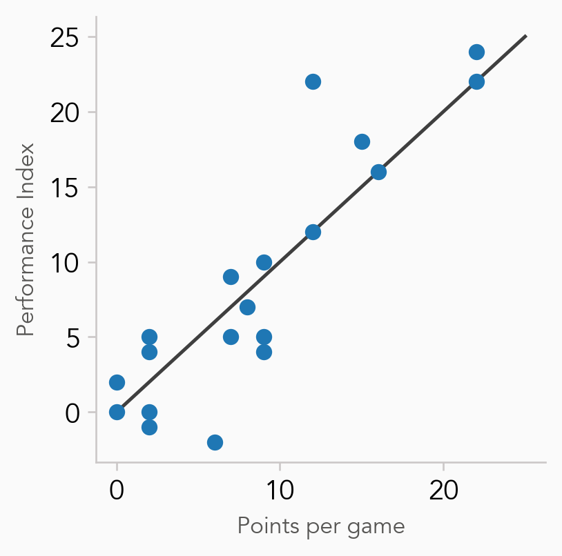
We could spend time making this plot look better if we were going to present it to others, for example, on social media, but here we are simply aiming to quickly inspect the data.

As the majority of the circles on the plot lie close to the y = x line, we can see that the Performance Index shows a pretty strong correlation with the points scored (which is one of the common criticisms of Performance Index). In other words, the trend in this data is that the Index isn’t really telling us much more than simply looking at the points scored.

What may be more useful here is to look at the difference between the Index and points scored, this will help us identify which players had a good game that wasn’t just scoring lots of points. We can do that through calculating a new column in the dataframe, which I will call “Diff” (for difference).

boxscores_df['Diff'] = boxscores_df['Index'] - boxscores_df['PTS']
boxscores_df['Diff'].describe()

count    19.000000
mean      0.000000
std       3.785939
min      -8.000000
25%      -2.000000
50%       0.000000
75%       2.000000
max      10.000000
Name: Diff, dtype: float64

We can see that one player had an Index that was ten points higher than the number of points scored, which means they made a big contribution in other ways than just scoring. Let’s ask the dataframe for any players who’s Index is greater than the number of points plus five (so we capture any other good performances).

boxscores_df[boxscores_df.Diff > 5.0]

	Name	Team	Mins	PTS	FGM	FGA	FG%	2PM	2PA	2P%	...	AST	TO	STL	BLK	BLKR	PF	FOULON	PLUSMINUS	Index	Diff
3	M. Washington	Hatters	31:36	12	6	9	66	6	9	66	...	4	3	5	1	0	2	2	13	22	10

1 rows × 29 columns

Okay, it’s pretty obvious in this case that Maddie Washington had the great performance, having a much bigger impact on the game than scoring 12 points would suggest.

While we are investigating this, let’s take a look at all the players with a positive “Diff”, and place them in order, so that the players with the highest Diff come first. If the Diff is the same, we order by Index.

boxscores_df[boxscores_df.Diff > 0.0].sort_values(['Diff', 'Index'], ascending=False)

	Name	Team	Mins	PTS	FGM	FGA	FG%	2PM	2PA	2P%	...	AST	TO	STL	BLK	BLKR	PF	FOULON	PLUSMINUS	Index	Diff
3	M. Washington	Hatters	31:36	12	6	9	66	6	9	66	...	4	3	5	1	0	2	2	13	22	10
2	N. Krisper	Hatters	33:37	15	6	10	60	5	7	71	...	5	5	2	0	0	3	3	10	18	3
4	E. Gandini	Hatters	20:30	2	1	4	25	1	2	50	...	1	1	0	0	0	1	1	10	5	3
17	D. Bryne	Gladiators	27:21	22	5	11	45	0	2	0	...	1	5	4	0	0	1	5	-4	24	2
5	M. Emanuel-Carr	Hatters	11:01	7	2	4	50	2	4	50	...	3	2	1	0	0	1	2	7	9	2
11	H. Robb	Gladiators	23:43	2	1	4	25	1	2	50	...	4	0	0	0	0	2	1	-15	4	2
15	R. Lewis	Gladiators	15:48	0	0	1	0	0	0	0	...	2	1	0	0	0	1	2	0	2	2
6	C. Drennan	Hatters	18:13	9	3	3	100	1	1	100	...	1	1	0	0	0	3	4	-2	10	1

8 rows × 29 columns

If we were to keep track of this Diff value over several games, it would help identify those players that consistently influence the game in ways that aren’t just points.

Of course, your team still needs scorers too!

Calculating the true shooting percentage

A common method for comparing how efficiently players shoot the ball is via the true shooting percentage. It considers all three types of shooting that appears in a boxscore (2 pointers, 3 pointers and free-throws) in the same metric. The common abbreviation used for true shooting is TS%.

\[\textrm{TS}\% = \frac{\textrm{PTS}}{2\left(\textrm{FGA} + \left(0.44 \times \textrm{FTA} \right) \right)}\]

To be able to analyse TS% for this game, let’s first define a function to calculate this “advanced stat”.

Note: If a player hasn't attempted any shots (field goals or free throws) then the above formula will attempt to divide the number of points by zero, which is mathematically undefined and will give an error. We will use some logic to return a TS% of zero in such cases.

def true_shooting(pts, fga, fta):
    if fga == 0 and fta == 0:
        ts = 0
    else:
        denominator = 2 * (fga + (0.44 * fta))
        ts = pts / denominator

    return ts

Now we use a lambda to compute this for all of the players in the dataframe.

boxscores_df['TS%'] = boxscores_df.apply(lambda x: true_shooting(x['PTS'], x['FGA'], 
                                                                 x['FTA']), axis=1)

As a first step in analysing this, we can compute the summary statistics of TS%, and look at a sorted slice of the dataframe.

boxscores_df['TS%'].describe()

count    19.000000
mean      0.532593
std       0.313783
min       0.000000
25%       0.369450
50%       0.531915
75%       0.672388
max       1.308140
Name: TS%, dtype: float64

boxscores_df[['Name', 'Team', 'TS%']].sort_values(['TS%'], ascending=False)

	Name	Team	TS%
6	C. Drennan	Hatters	1.308140
14	K. Brown	Gladiators	1.000000
17	D. Bryne	Gladiators	0.757576
2	N. Krisper	Hatters	0.689338
1	G. Gayle	Hatters	0.675676
13	K. Tudor	Gladiators	0.669100
3	M. Washington	Hatters	0.666667
5	M. Emanuel-Carr	Hatters	0.657895
0	L. Zolper	Hatters	0.541516
18	K. Mcghee	Gladiators	0.531915
10	M. Domenger	Gladiators	0.515464
9	L. Wright-Ponder	Hatters	0.436047
16	T. Adams	Gladiators	0.431034
8	S. Harrison	Hatters	0.414692
12	E. Mcgarrachan	Gladiators	0.324207
11	H. Robb	Gladiators	0.250000
4	E. Gandini	Hatters	0.250000
7	E. Nibbelink	Hatters	0.000000
15	R. Lewis	Gladiators	0.000000

A first reaction here may be “wow, a player has a true shooting percentage of 130%, how does this make sense?”. There are (at least) two things going on here. The first is that TS% can give values of greater than 100%, which is a minor problem with this particular stat, and the second is that a single game is a very small sample size, where “outliers” like this are more likely to happen.

Still, it looks like Carla Drennan of the Hatters had an excellent game in terms of shooting. By looking at a subset of their game stats, we can confirm that.

boxscores_df[['Name', 'Team', 'PTS', 'FGM', 'FGA', 'FG%', '3PM', '3PA', '3P%',
             'FTA', 'FTM', 'FT%', 'TS%']].loc[boxscores_df['Name'] == 'C. Drennan']

	Name	Team	PTS	FGM	FGA	FG%	3PM	3PA	3P%	FTA	FTM	FT%	TS%
6	C. Drennan	Hatters	9	3	3	100	2	2	100	1	1	100	1.30814

Now we see that Carla had a perfect shooting night, scoring every 3 pointer (2 of them), 2 pointer (1 of them), and free throw (1 of them) attempted. As they made all of the shots, and some of them were 3 pointers, this explains the TS% that is greater than 100.

It’s important to consider the shot volume (how many shots have been attempted) as well as the efficiency - you can think of this in terms of getting the hot hand the ball.

Note: Dean Oliver's book "Basketball on paper" has a fascinating chapter on whether or not the "hot hand" actually exists, well worth a read. I often wish that I'd become familiar with Oliver's ideas a lot sooner - I was playing for a university team 20 years ago when the book was originally published and the approaches and ideas presented would have shaped my thinking about the game. Sometimes I wonder if I would have pursued sports analytics as a carrer, if I'd have known about it.

This is best visualised as a plot of TS% against field goal attempts.

Note: The FGA doesn't account for free throws. It probably doesn't matter too much here, but in principle one could design some sort of weighted shots metric that accounts for FTA (and possibly weights 2PT and 3PT differently). Another alternative could be to consider "Usage", but I will leave that for another Chapter.

plt.rcParams.update({'font.family':'Avenir'})
bgcol = '#fafafa'

fig, ax = plt.subplots(figsize=(3.5, 3.5), dpi=240)
fig.set_facecolor(bgcol)
ax.set_facecolor(bgcol)
ax.scatter(boxscores_df['FGA'], boxscores_df['TS%'])

ax.spines['right'].set_visible(False)
ax.spines['top'].set_visible(False)
ax.spines['left'].set_color('#ccc8c8')
ax.spines['bottom'].set_color('#ccc8c8')

plt.tick_params(axis='x', labelsize=12, color='#ccc8c8')
plt.tick_params(axis='y', labelsize=12, color='#ccc8c8')

plt.xlabel('Field Goal Attempts', color='#575654')
plt.ylabel('True Shooting Percentage', color='#575654');

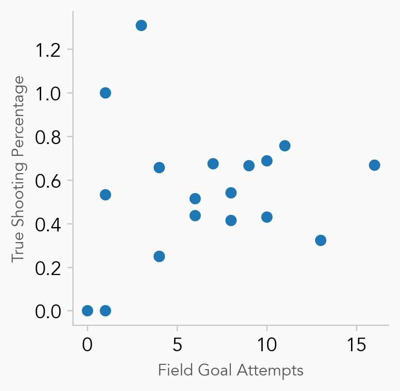
There’s probably too many points here and it distracts from the analysis we want - in this case, players with a good TS% and reasonable volume of shots. Here I will create a new dataframe that only contains the players who took more than 2 shots and have a TS% between 0.5 and 1.0 (we already know that Drennan was perfect from the floor).

shooters_df = boxscores_df[(boxscores_df.FGA > 2) & (boxscores_df["TS%"] > 0.5) & 
    (boxscores_df["TS%"] <= 1.0)]
shooters_df.reset_index(drop=True, inplace=True)
len(shooters_df)

8

That’s left us with 8 players, so let’s plot that again. We will also add the player names as annotations to the points.

plt.rcParams.update({'font.family':'Avenir'})
bgcol = '#fafafa'

fig, ax = plt.subplots(figsize=(3.5, 3.5), dpi=240)
fig.set_facecolor(bgcol)
ax.set_facecolor(bgcol)
ax.scatter(shooters_df['FGA'], shooters_df['TS%'])

ax.spines['right'].set_visible(False)
ax.spines['top'].set_visible(False)
ax.spines['left'].set_color('#ccc8c8')
ax.spines['bottom'].set_color('#ccc8c8')

plt.tick_params(axis='x', labelsize=12, color='#ccc8c8')
plt.tick_params(axis='y', labelsize=12, color='#ccc8c8')

plt.xlabel('Field Goal Attempts', color='#575654')
plt.ylabel('True Shooting Percentage', color='#575654')

for idx, row in shooters_df.iterrows():
    ax.annotate(row['Name'], (row['FGA'], row['TS%']), 
                xytext=(4.5, -2.5), textcoords='offset points')

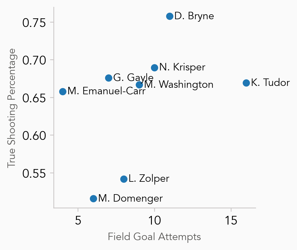
There’s a “seam” of good shooting performances with a TS% greater than 0.65 and decent volume. The ideal here is for players to be in the upper right corner and that allows us to identify Delaynie Bryne and Katharine Tudor as two of the top shooting performers in this game.

Repeating this type of analysis for a team over several games allows the statistical outlier performances to “regress to the mean” and the real true shooters to be identified.

Exercises

To help solidify these concepts and the mechanics of how to calculate them, it’s a good idea to practise them a bit by repeating the exercise.

1. Load the boxscore data for a different game into a dataframe (this could be an existing CSV file, or you could flex your Python muscles and scrape a new one.

2. Calculate the Performance Index and TS% for all of the players who saw game time.

3. Analyse the data to identify players who played well beyond just scoring points, and those who had the best shooting nights (don’t forget to account for the volume of shots in addition to accuracy).

Team-level stats

When looking at player-level stats, they are automatically “normalised” by virtue of them being “per game”. However, we sometimes also normalise by looking at what the contribution would have been if the player had played for 40 minutes (“per 40”), giving some insights into how a given player who didn’t play for large stretches of the game might have done if they saw more court time.

For some team-level stats, it will be useful to know how much time was played in total (team minutes). While for a normal game this will be 200 minutes (40 minutes for 5 players), if we want to have workflows that work for any game we also need to account for overtime. The first step in this is to convert the Minutes:Seconds format of the time to be in seconds.

def get_total_seconds(stringMS):
    time_Obj = dt.datetime.strptime(stringMS, "%M:%S") - dt.datetime(1900,1,1)
    return time_Obj.total_seconds()

boxscores_df['Seconds'] = boxscores_df.apply(lambda x: get_total_seconds(x['Mins']), axis=1)

We can pull out the relevant columns from the dataframe to make sure this looks sensible.

boxscores_df[['Name', 'Team', 'Seconds']]

	Name	Team	Seconds
0	L. Zolper	Hatters	1740.0
1	G. Gayle	Hatters	1435.0
2	N. Krisper	Hatters	2017.0
3	M. Washington	Hatters	1896.0
4	E. Gandini	Hatters	1230.0
5	M. Emanuel-Carr	Hatters	661.0
6	C. Drennan	Hatters	1093.0
7	E. Nibbelink	Hatters	317.0
8	S. Harrison	Hatters	1041.0
9	L. Wright-Ponder	Hatters	570.0
10	M. Domenger	Gladiators	1367.0
11	H. Robb	Gladiators	1423.0
12	E. Mcgarrachan	Gladiators	1872.0
13	K. Tudor	Gladiators	1841.0
14	K. Brown	Gladiators	1277.0
15	R. Lewis	Gladiators	948.0
16	T. Adams	Gladiators	1296.0
17	D. Bryne	Gladiators	1641.0
18	K. Mcghee	Gladiators	335.0

We will come back to these times a little later. When we look at team-level stats for a given game, it can be useful to normalise them in a different way than the “per 40” than they already are (assuming no overtime). This leads us to…

Possessions

The concept of breaking the game down into “possessions” has been around a long time, with Dean Oliver mentioning that he saw it in a book by Frank McGuire (interestingly, Oliver mentions that he originally thought he’d invented the concept until he found it elsewhere). The general principle is that a team alternates possessions with the opponent and the two teams will end up with roughly the same number of possessions over the course of a game. It is not simply the number of shots as it needs to account for offensive rebounds (i.e., the team on offence still has possession), turnovers commited etc. The number of possessions in a game will also give you some indication of the pace of play - teams playing fast end up with a lot of possessions.

There are various formulae used to estimate the number of possessions based on team-level stats, with varying degress of complexity. The one we will use here is:

\[\mathrm{Possessions} = 0.96 \times \left(\mathrm{FGA} + \mathrm{TO} + 0.44 \times \mathrm{FTA} - \mathrm{OREB}\right)\]

To be able to calculate this, we are going to need to sum the player-level stats on a per-team basis.

Some of the data we gather here will be used later, so stick with it if it doesn’t seem totally obvious at this point. We start by creating individual dataframes for each team by pulling out the relevant rows of the boxscores.

hatters_df = boxscores_df[boxscores_df['Team'] == 'Hatters']
glads_df = boxscores_df[boxscores_df['Team'] == 'Gladiators']

We can then use the pandas “sum” function to calculate the totals we need for both teams. This is a bit convoluted, but we start by defining which columns we want.

column_list = ['Seconds', 'PTS', 'FGA', 'TO', 'FTA', 'OREB']

We then sum these columns and add them to a dictionary for each team. We also add the team names and the number of points allowed (that is, how many points the other team scored) to these dictionaries.

hatters_totals = hatters_df[column_list].sum().to_dict()
hatters_totals['Team'] = 'Hatters'
glads_totals = glads_df[column_list].sum().to_dict()
glads_totals['Team'] = 'Gladiators'

hatters_totals['PTS_Allowed'] = glads_totals['PTS']
glads_totals['PTS_Allowed'] = hatters_totals['PTS']

We then combine the dictionaries into a list of dictionaries and then convert that into dataframe

totals=[hatters_totals, glads_totals]
totals_df = pd.DataFrame(totals)

Now we re-arrange the dataframe and see what it looks like.

totals_df = totals_df[['Team', 'Seconds', 'PTS', 'PTS_Allowed','FGA', 'TO', 'FTA', 'OREB']]
totals_df

	Team	Seconds	PTS	PTS_Allowed	FGA	TO	FTA	OREB
0	Hatters	12000.0	86.0	76.0	59.0	21.0	27.0	9.0
1	Gladiators	12000.0	76.0	86.0	63.0	21.0	18.0	13.0

The seconds part looks a bit odd, so let’s convert that back to the Mins:Secs format now that it has been summed.

def seconds_to_minsseconds(seconds):
    return '{}:{}'.format(*divmod(int(seconds), 60))

totals_df['Mins'] = totals_df.apply(lambda x: seconds_to_minsseconds(x['Seconds']), axis=1)
totals_df = totals_df[['Team', 'Mins', 'PTS', 'PTS_Allowed','FGA', 'TO', 'FTA', 'OREB']]

totals_df

	Team	Mins	PTS	PTS_Allowed	FGA	TO	FTA	OREB
0	Hatters	200:0	86.0	76.0	59.0	21.0	27.0	9.0
1	Gladiators	200:0	76.0	86.0	63.0	21.0	18.0	13.0

That looks better, each team has played the 200 minutes we would expect for a normal length game (no O/T).

We now define a function to calculate the number of possessions.

def possessions(fga, to, fta, oreb):
    possessions = 0.96 * (fga + to + 0.44*fta - oreb)

    return possessions

As we’ve done a few times, now use a lambda to calculate this for both teams.

totals_df['Possessions'] = totals_df.apply(lambda x: possessions(x['FGA'], x['TO'], 
                                            x['FTA'], x['OREB']), axis=1)

Let’s take a look at the results.

totals_df

	Team	Mins	PTS	PTS_Allowed	FGA	TO	FTA	OREB	Possessions
0	Hatters	200:0	86.0	76.0	59.0	21.0	27.0	9.0	79.5648
1	Gladiators	200:0	76.0	86.0	63.0	21.0	18.0	13.0	75.7632

We can see that the Hatters had slightly more estimated possessions, which seems to have come from the number of trips to the free-throw line they had.

Offensive efficiency rating

The offensive efficiency rating, or OER, is the number of points the team scored per 100 possessions.

def oer(pts, possessions):
    return 100 * (pts/possessions)

totals_df['OER'] = totals_df.apply(lambda x: oer(x['PTS'], 
                                            x['Possessions']), axis=1)

totals_df

	Team	Mins	PTS	PTS_Allowed	FGA	TO	FTA	OREB	Possessions	OER
0	Hatters	200:0	86.0	76.0	59.0	21.0	27.0	9.0	79.5648	108.087999
1	Gladiators	200:0	76.0	86.0	63.0	21.0	18.0	13.0	75.7632	100.312553

This shows us that the Hatters scored 108 points per 100 possessions, where the Gladiators scored 100. Interestingly, basketball is a game where usually a team scores an average of about 1 point per possession. This leads to lots of analysis of how many points a player scores on different types of possession, for example how many on average do they score per post-up.

However, we’re looking at team-level stats here, so let’s not get too distracted.

Defensive efficiency rating

Perhaps unsurprisingly, the defensive efficiency rating (DER) is the number of points allowed per 100 possessions.

def der(pts_allowed, possessions):
    return 100 * (pts_allowed/possessions)

totals_df['DER'] = totals_df.apply(lambda x: der(x['PTS_Allowed'], 
                                            x['Possessions']), axis=1)

totals_df

	Team	Mins	PTS	PTS_Allowed	FGA	TO	FTA	OREB	Possessions	OER	DER
0	Hatters	200:0	86.0	76.0	59.0	21.0	27.0	9.0	79.5648	108.087999	95.519627
1	Gladiators	200:0	76.0	86.0	63.0	21.0	18.0	13.0	75.7632	100.312553	113.511573

Rather than analysing the DER, we can jump straight to an overall rating.

Net rating

The net rating (NET) is simply the difference between OER and DER.

def net(oer, der):
    return oer - der

totals_df['NET'] = totals_df.apply(lambda x: net(x['OER'], 
                                            x['DER']), axis=1)

totals_df

	Team	Mins	PTS	PTS_Allowed	FGA	TO	FTA	OREB	Possessions	OER	DER	NET
0	Hatters	200:0	86.0	76.0	59.0	21.0	27.0	9.0	79.5648	108.087999	95.519627	12.568372
1	Gladiators	200:0	76.0	86.0	63.0	21.0	18.0	13.0	75.7632	100.312553	113.511573	-13.199020

It’s probably best not to read too much into this, but the NET ratings do suggest that if the game had been 100 possessions, the Hatters should have won by about 13 points (rather than the 10 points from 76 to 80 possessions).

Once you start to average NET over several games, it should give an idea of which teams are playing well, and which are not. As a basic “rule-of-thumb”, teams with a positive net rating are “good” and those with a negative rating are not.

Pace

Pace is the total number of possessions each team uses in a game - as the name suggests, it gives an indication of how quick the team is playing and is another statistic that makes more sense to average over multiple games.

It is calculated as:

\[\mathrm{Pace} = \frac{200}{\mathrm{Team Mins}} \times \frac{\mathrm{Possessions} + \mathrm{Opponent Possessions}}{2}\]

Inspecting the equation tells us that the first term accounts for any overtime played, while the second takes the average of the game’s possessions. It’s also clear the the pace will be the same for both teams in a given game.

We can work it out as a single calculation, rather than defining a function.

pace = (200 / int(totals_df.iloc[0]['Mins'].split(':')[0])) * ((totals_df.iloc[0]['Possessions'] + totals_df.iloc[1]['Possessions']) / 2)
pace

77.66399999999999

To add this to the dataframe, we create a list that contains the pace twice (once for each team), then add the list to the dataframe as a new column.

pace_list = [pace, pace]
totals_df['Pace'] = pace_list
totals_df

	Team	Mins	PTS	PTS_Allowed	FGA	TO	FTA	OREB	Possessions	OER	DER	NET	Pace
0	Hatters	200:0	86.0	76.0	59.0	21.0	27.0	9.0	79.5648	108.087999	95.519627	12.568372	77.664
1	Gladiators	200:0	76.0	86.0	63.0	21.0	18.0	13.0	75.7632	100.312553	113.511573	-13.199020	77.664

As you can probably tell, pace is a stat that should be tracked over the course of several games as it doesn’t provide many performance insights on its own.

Exercises

1. We will get slightly different values of OER, DER and NET if we round the value of Possessions so that it’s an integer. You could explore round the value using the floor, ceiling and round functions to see how it changes things.

2. There’s a more complicated version of the formula for calculating the number of possessions, which is given in Oliver’s Basketball on Paper. Try using the formula below to see if it produces a noticeable difference in OER, DER and NET.

\[\mathrm{Possessions} = \mathrm{FGA} - \frac{\mathrm{OREB}}{\mathrm{OREB} + \mathrm{DDREB}} \times \left(\mathrm{FGA} - \mathrm{FGM}\right) \times 1.07 + \mathrm{TO} + 0.4 \times \mathrm{FTA}\]

where \(\mathrm{DDREB}\) is the number of defensive rebounds that the opposition recorded.